Gnocchi 使用原理及源码分析-下

任何你的不足,在你成功的那刻,都会被人说为特色。所以,坚持做你自己,而不是在路上被别人修改的面目全非。

继续上篇的内容之前,先介绍下和今天有关系的两个库 numpy 、 pandas

工具

pandas

简介

Python Data Analysis Library 或 pandas 是基于NumPy 的一种工具,该工具是为了解决数据分析任务而创建的。Pandas 纳入了大量库和一些标准的数据模型,提供了高效地操作大型数据集所需的工具。pandas提供了大量能使我们快速便捷地处理数据的函数和方法。你很快就会发现,它是使Python成为强大而高效的数据分析环境的重要因素之一。

Pandas 是python的一个数据分析包,最初由AQR Capital Management于2008年4月开发,并于2009年底开源出来,目前由专注于Python数据包开发的PyData开发team继续开发和维护,属于PyData项目的一部分。Pandas最初被作为金融数据分析工具而开发出来,因此,pandas为时间序列分析提供了很好的支持。 Pandas的名称来自于面板数据(panel data)和python数据分析(data analysis)。panel data是经济学中关于多维数据集的一个术语,在Pandas中也提供了panel的数据类型。

数据结构

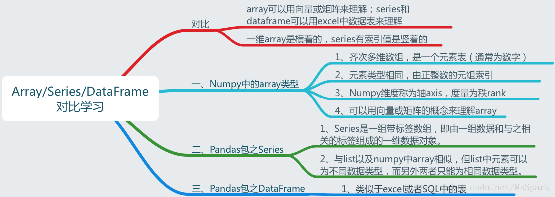
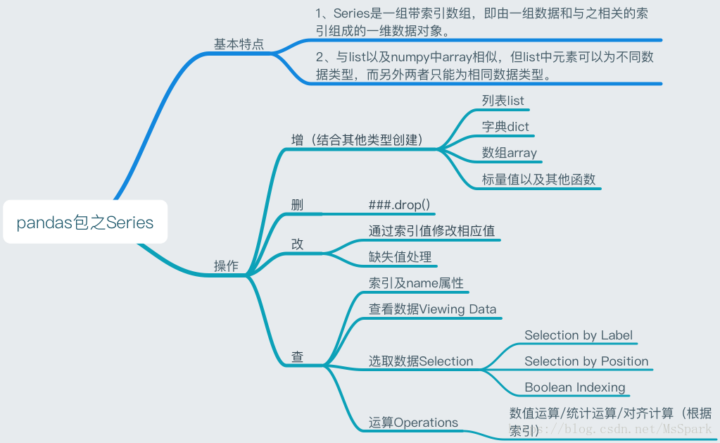
Series:一维数组,与Numpy中的一维array类似。二者与Python基本的数据结构List也很相近,其区别是:List中的元素可以是不同的数据类型,而Array和Series中则只允许存储相同的数据类型,这样可以更有效的使用内存,提高运算效率。以下内容基本以这种结构为主。

Time- Series:以时间为索引的Series。

DataFrame:二维的表格型数据结构。很多功能与R中的data.frame类似。可以将DataFrame理解为Series的容器。

Panel :三维的数组,可以理解为DataFrame的容器。

Pandas 有两种自己独有的基本数据结构。读者应该注意的是,它固然有着两种数据结构,因为它依然是 Python 的一个库,所以,Python 中有的数据类型在这里依然适用,也同样还可以使用类自己定义数据类型。只不过,Pandas 里面又定义了两种数据类型:Series 和 DataFrame,它们让数据操作更简单了。

使用 Series

创建 series

1
2
3
4
5
6
7
8
9
10
11
12
13
14
15
16
17
18
19
20
21
22
23
24
25
26
27
28
29
30
31
32
33
34
35
36
#导入 Pandas 包
import pandas as pd

#创建Series
#1.1.1 通过列表 List
listSer=pd.Series([10,20,30,40])
print(listSer)

#1.1.2 通过字典 dict
dictSer=pd.Series({'a':10,'b':40,'c':5,'d':90,'e':35,'f':40},name='数值')
print(dictSer)

#1.1.3 通过 array
import numpy as np
arrySer=pd.Series(np.arange(10,15),index=['a','b','c','d','e'])
print(arrySer)

[output]
0 10
1 20
2 30
3 40
dtype: int64
a 10
b 40
c 5
d 90
e 35
f 40
Name: 数值, dtype: int64
a 10
b 11
c 12
d 13
e 14
dtype: int64

index及value属性

1
2
3
4
5
6
7
8
9
10
# Series类型包括(index,values)两部分

#index
print(arrySer.index)
#values
print(arrySer.values)

[output]
Index(['a', 'b', 'c', 'd', 'e'],dtype='object')
[10 11 12 13 14]
1
2
3
4
5
6
7
8
9
10
11
12
pandas.Index.is_monotonic # Alias for is_monotonic_increasing

pandas.Index.is_monotonic_increasing
# Return if the index is monotonic increasing (only equal or increasing) values.

# example
Index([1, 2, 3]).is_monotonic_increasing
True
Index([1, 2, 2]).is_monotonic_increasing
True
Index([1, 3, 2]).is_monotonic_increasing
False
1
2
3
4
5
6
7
8
9
10
pandas.Index.has_duplicates
# Check if the Index has duplicate values.

idx = pd.Index([1, 5, 7, 7])
idx.has_duplicates
True

idx = pd.Index([1, 5, 7])
idx.has_duplicates
False
1
2
3
4
5
6
7
8
9
10
11
12
13
14
15
16
17
18
19
20
21
22
pandas.Series.combine_first(other)
# 用“other”中相同位置的值更新空元素。
# 通过用另一个系列的非空值填充一个系列中的空值来组合两个系列对象。结果索引将是两个索引的并集。

# example
s1 = pd.Series([1, np.nan])
s2 = pd.Series([3, 4, 5])
s1.combine_first(s2)
0 1.0
1 4.0
2 5.0
dtype: float64


# 如果该空值的位置不存在于 other
s1 = pd.Series({'falcon': np.nan, 'eagle': 160.0})
s2 = pd.Series({'eagle': 200.0, 'duck': 30.0})
s1.combine_first(s2)
duck 30.0
eagle 160.0
falcon NaN
dtype: float64

pandas methed

获取数据

1
2
3
4
5
6
7
8
9
10
11
12
13
14
15
16
17
18
19
20
21
22
23
24
25
26
27
28
#iloc通过位置获取数据
dictSer[0:1] #相当于dictSer.iloc[0:1]
>>>
a 10
Name: 数值, dtype: int64

#loc通过索引获取数据
dictSer[['a','b']] #相当于dictSer.loc[['a','b']]
>>>
a 10
b 40
Name: 数值, dtype: int64

#boolean indexing获取值
dictSer[dictSer.values<=10] #获取值不超过10的数据
>>>
a 10
c 5
Name: 数值, dtype: int64

dictSer[dictSer.index!='a'] #获取索引值不是a的数据
>>>
b 40
c 5
d 90
e 35
f 40
Name: 数值, dtype: int64

基本运算

1
2
3
4
5
6
7
8
9
10
11
12
13
14
15
16
17
18
19
20
# 查看描述性统计数据

dictSer.describe()
>>>
count 6.000000
mean 36.666667
std 30.276504
min 5.000000
25% 16.250000
50% 37.500000
75% 40.000000
max 90.000000
Name: 数值, dtype: float64

dictSer.mean() #均值
dictSer.median() #中位数
dictSer.sum() #求和
dictSer.std() #标准差
dictSer.mode() #众数
dictSer.value_counts() #每个值的数量
1
2
3
4
5
6
7
8
# 数学运算

dictSer/2 #对每个值除2
dictSer//2 #对每个值除2后取整
dictSer%2 #取余
dictSer**2 #求平方
np.sqrt(dictSer) #求开方
np.log(dictSer) #求对数
1
2
3
4
5
6
7
8
9
10
11
12
13
14
15
16
# 对齐计算

dictSer2=pd.Series({'a':10,'b':20,'d':23,'g':90,'h':35,'i':40},name='数值')
dictSer3=dictSer+dictSer2
dictSer3
>>>
a 20.0
b 60.0
c NaN
d 113.0
e NaN
f NaN
g NaN
h NaN
i NaN
Name: 数值, dtype: float64

缺失值处理

1
2
3
4
5
6
7
8
9
10
11
12
13
14
15
16
17
18
19
20
21
22
23
24
25
26
27
28
29
30
31
#找出空/非空值
dictSer3[dictSer3.notnull()] #非空值
>>>
a 20.0
b 60.0
d 113.0
Name: 数值, dtype: float64

dictSer3[dictSer3.isnull()] #空值
>>>
c NaN
e NaN
f NaN
g NaN
h NaN
i NaN
Name: 数值, dtype: float64

#填充空值
dictSer3=dictSer3.fillna(dictSer3.mean()) #用均值来填充缺失值
>>>
a 20.000000
b 60.000000
c 64.333333
d 113.000000
e 64.333333
f 64.333333
g 64.333333
h 64.333333
i 64.333333
Name: 数值, dtype: float64

删除值

1
2
3
4
5
6
7
8
9
10
11
12
dictSer3=dictSer3.drop('b')
print(dictSer3)
>>>
a 20.000000
c 64.333333
d 113.000000
e 64.333333
f 64.333333
g 64.333333
h 64.333333
i 64.333333
Name: 数值, dtype: float64

总结归纳:

Array/Series/DataFrame对比学习

Pandas包之Series

使用 timestamp

Timestamp()

1
2
3
4
5
6
7
8
9
10
11
12
13
14
15
16
17
18
19
20
import pandas as pd
from datetime import datetime as dt
p1=pd.Timestamp(2017,6,19)
p2=pd.Timestamp(dt(2017,6,19,hour=9,minute=13,second=45))
p3=pd.Timestamp("2017-6-19 9:13:45")

print("type of p1:",type(p1))
print(p1)
print("type of p2:",type(p2))
print(p2)
print("type of p3:",type(p3))
print(p3)

输出:
('type of p1:', <class 'pandas.tslib.Timestamp'>)
2017-06-19 00:00:00
('type of p2:', <class 'pandas.tslib.Timestamp'>)
2017-06-19 09:13:45
('type of p3:', <class 'pandas.tslib.Timestamp'>)
2017-06-19 09:13:45

to_datetime()

pandas.to_datetime(arg,errors ='raise',utc = None,format = None,unit = None )

errors:三种取值,‘ignore’, ‘raise’, ‘coerce’,默认为raise。

  • ‘raise’,则无效的解析将引发异常

  • ‘coerce’,那么无效解析将被设置为NaT

  • ‘ignore’,那么无效的解析将返回输入值

utc:布尔值,默认为none。返回utc即协调世界时。
format:格式化显示时间的格式。
unit:默认值为‘ns’,则将会精确到微妙,‘s’为秒。

1
2
3
4
5
6
7
8
9
10
11
12
13
14
15
16
import pandas as pd
from datetime import datetime as dt

p4=pd.to_datetime("2017-6-19 9:13:45")
p5=pd.to_datetime(dt(2017,6,19,hour=9,minute=13,second=45))

print("type of p4:",type(p4))
print(p4)
print("type of p5:",type(p5))
print(p5)

输出:
('type of p4:', <class 'pandas.tslib.Timestamp'>)
2017-06-19 09:13:45
('type of p5:', <class 'pandas.tslib.Timestamp'>)
2017-06-19 09:13:45

numpy

Numpy(Numerical Python 的简称)时高性能科学计算和数据分析的基础包,提供了矩阵运算的功能。

相关链接Numpy官方推荐教程

Numpy具有以下几点能力:

  • ndarry——一个具有向量算数运算和复杂广播能力的多位数组对象
  • 用于对数组数据进行快速运算的标准数学函数
  • 用于读写磁盘数据的工具以及用于操作内存映射文件的工具
  • 非常有用的线性代数,傅立叶变换和随机数操作
  • 用于继承c/c++和Fortran代码的工具

创建Numpy数组

1
2
3
4
5
6
7
8
9
10
11
12
13
# 使用numpy.array()可直接导入数组或矩阵

import numpy as np
a = np.array([1,2,3,4,5])
b = np.array([[1,1,1],[2,2,2],[3,3,3]])
print(a)
print(b)

# 结果
[1 2 3 4 5]
[[1 1 1]
[2 2 2]
[3 3 3]]

获取与创建数组时设置纬度

1
2
3
4
5
6
7
8
9
10
11
12
13
14
15
16
17
# reshape将当前一位数组设置成对应的m*n的矩阵

a = np.array([1,2,3,4,5,6,7,8,9,10,11,12,13,14,15])
a = a.reshape(3,5)
print(a)

# 结果
[[ 1 2 3 4 5]
[ 6 7 8 9 10]
[11 12 13 14 15]]

# 通过a.shape()可以查看当前矩阵的纬度,返回值是一个元组

tu = a.shape
print(tu)
# 结果
(3, 5)

数组索引、切片、比较

1
2
3
4
5
6
7
8
9
10
11
12
13
14
15
16
17
18
19
20
21
22
23
24
25
26
27
matrix = np.array([[1,2,3],[20,30,40]])
# *索引与正常二位数组相同*
print(matrix[0,1])
matrix = np.array([
[5,10,15],
[20,25,30],
[35,40,45]])
# *切片与正常二维数组相同*
print(matrix[:,1])
print(matrix[:,0:2])
print(matrix[1:3,:])
print(matrix[1:3,0:2])
# *结果*
2
[10 25 40]
[[ 5 10]
[20 25]
[35 40]]
[[20 25 30]
[35 40 45]]
[[20 25]
[35 40]]
# *比较返回的是每一个数组元素比较之后的值,返回的也是一个数组,都是布尔类型*
z = (matrix[1,:]==25)
print(z)
# *结果*
[False True False]

数组值的替换

值的替换在自然语言处理中很有用,例如我们在处理一个文本数组的时候,有几个数据元素是空,那么我们可以结合判断语句来获得是否为空的一个布尔数组,然后利用这个布尔数组进行元素替换

1
2
3
4
5
6
matrix=np.array([['1','2',''],['3','4','5'],['5','6','']])
m = (matrix[:,2] == '')
matrix[m,2]='0'
print(matrix)

# *这里判断第三列中值为空的数据,返回一个bool类型的数组,再将bool类型的数组当成是数组的下标进行替换数据就可以了,这里只会替换值为真的时候的值,所以完全不必担心替换不必要的数据*

数据类型转换

初始化时设置数据类型用dtype
astype用于更改数据类型

1
2
3
4
5
vector = np.array(['1','2','3'])
vector = vector.astype(float)
print(vector)
*结果*
[1. 2. 3.]

统计计算方法

1
2
3
4
5
6
7
8
9
10
11
12
13
14
15
16
17
18
19
20
21
sum
mean
max
**********
vector.sum()
vector.mean()
vector.max()
**********
6.0
2.0 平均
3.0 最大
************
对于矩阵需要设置行或者列
matrix = np.array([[20,10,15],[30,20,14],[30,29,43]])
matrix.sum(axis=1)//每行相加求和
*结果*
array([ 45, 64, 102])

matrix.sum(axis=0)//每列相加求和
*结果*
array([80, 59, 72])

计算差值

numpy.diff(a, n=1,axis=-1)

沿着指定轴计算第N维的离散差值
参数:
a:输入矩阵
n:可选,代表要执行几次差值
axis:默认是最后一个
示例:

1
2
3
4
5
6
7
8
9
10
11
12
13
14
15
import numpy as np

A = np.arange(2 , 14).reshape((3 , 4))
A[1 , 1] = 8
print('A:' , A)
# A: [[ 2 3 4 5]
# [ 6 8 8 9]
# [10 11 12 13]]

print(np.diff(A))
# [[1 1 1]
# [2 0 1]
# [1 1 1]]

# 从输出结果可以看出,其实diff函数就是执行的是后一个元素减去前一个元素。

添加元素 insert

numpy.insert(arr, obj, values, axis=None)

第一个参数arr是一个数组,可以是一维的也可以是多维的,在arr的基础上插入元素

第二个参数obj是元素插入的位置

第三个参数values是需要插入的数值

第四个参数axis是指示在哪一个轴上对应的插入位置进行插入

1
2
3
4
5
6
7
8
9
10
11
12
13
14
15
16
# 一维数组示例

import numpy as np

a = np.arange(4)
print(a)
# [0 1 2 3]

print(np.insert(a, 2, 100))
# [ 0 1 100 2 3]

print(np.insert(a, 1, [100, 101, 102]))
# [ 0 100 101 102 1 2 3]

print(np.insert(a, [0, 2, 4], [100, 101, 102]))
# [100 0 1 101 2 3 102]

多维数组可以看下 –> numpy.insert 详解

缓冲区读取

numpy.frombuffer(buffer, dtype = float, count = -1, offset = 0)

第一个参数 bufferbuffer_like:公开缓冲区接口的对象。

第二个参数 dtypedata-type, 可选:返回array的数据类型;默认值:float。

第三个参数 countint, 可选:要阅读的条目数。-1表示缓冲区中的所有数据。

第四个参数 offsetint, 可选:从这个偏移量(以字节为单位)开始读取缓冲区;默认值:0

此函数将缓冲区解释为一维数组。 暴露缓冲区接口的任何对象都用作参数来返回ndarray

1
2
3
4
5
6
7
import numpy as np 
s = 'Hello World'
a = np.frombuffer(s, dtype = 'S1')
print a

# 输出
# ['H' 'e' 'l' 'l' 'o' ' ' 'W' 'o' 'r' 'l' 'd']

计算给定轴上数组元素的累计和

numpy.cumsum(arr, axis=None, dtype=None, out=None)

第一个参数 arr : [数组]包含需要累计综合的数字的数组。如果arr不是数组,则尝试进行转换。

第二个参数 axis : 计算累计的轴,默认值是计算展平数组的综合。

  • axis=0,按照行累加。
  • axis=1,按照列累加。
  • axis不给定具体值,就把numpy数组当成一个一维数组。

第三个参数 dtype : 返回数组的类型,以及与元素相乘的累加器的类型。如果未指定dtype,则默认为arr的dtype,除非arr的整数dtype的精度小于默认平台整数的精度。在这种情況下,将使用默认平台整数。

第四个参数 out :[ndarray,可选]将结果存储到的位置。

  • 如果提供,则必須具有广播输入的形狀。
  • 如果未提供或沒有,则返回新分配的数组。

返回 Return :除非指定out,否则将返回保存结果的新数组,在这种情況下将返回该数组。

1
2
3
4
5
6
7
8
9
10
11
12
13
14
15
16
17
18
19
20
21
22
23
24
25
26
27
28
29
30
31
a = np.array([[1,2,3], [4,5,6]])

np.cumsum(a)
# array([ 1, 3, 6, 10, 15, 21])

#按照行累加,行求和
np.cumsum(a,axis=0)

array([[1, 2, 3],

[5, 7, 9]])

[1, 2, 3]------> |1 |2 |3 |

[4, 5, 6]------> |5=1+4 |7=2+5 |9=3+6|

#按照列累加,列求和
np.cumsum(a,axis=1)
array([[ 1, 3, 6],

[ 4, 9, 15]])
[1, 2, 3]------> |1 |2+1 |3+2+1 |

[4, 5, 6]------> |4 |4+5 |4+5+6 |

# 指定输出类型
np.cumsum(a, dtype=float)
# 注意啦!没有指定轴参数(axis)!输出就变成1维数组了。
array([ 1., 3., 6., 10., 15., 21.])第一步:每个值都变成float了

array([11+2=31+2+3=61+2+3+4=101+2+3+4+5=151+2+3+4+5+6=21])第二部:累加

Numpy官方推荐教程

上述两个库的体量很大,这里只是简单介绍,有兴趣的同学可自行 google

struct

python中struct 模块用于python数据结构与C结构之间的相互转换,其中C结构是用一种格式化字符串表示的,学习struct 模块的难点就在这个格式化字符串上

常见方法

1
2
3
4
5
6
7
8
9
10
11
12
13
14
# 常见方法

#将v1 v2按照fmt 转化为一个字节流(bytes)
struct.pack(fmt, v1, v2, ...)
#将v1 v2按照fmt 转化为一个字节流(bytes),并写入buffer,从位置offset处开始写入
struct.pack_into(fmt, buffer, offset, v1, v2, ...)
#将字节流按照fmt转化为python对象返回
struct.unpack(fmt, string)
#同unpack,只是针特定buffer转化为python对象返回
struct.unpack_from(fmt, buffer[, offset=0])
#返回fmt的所表示的C结构体所占字节大小
struct.calcsize(fmt)
#如果一述函数使用过程中fmt格式不对,会抛出这个异常
exception struct.error

格式化串

格式化串的字符根据功能不同可以分为两类,一类用于控制字节顺序、大小及对齐(Byte Order, Size, and Alignment),另一类用于表示结构体的组成(Format Characters)。

Byte Order, Size, and Alignment

字节顺序对齐相关知识详见 C语言字节对齐问题详解(对齐、字节序、网络序等)

字符 字节序 大小 对齐方式
@ 原生 原生 原生
= 原生 标准
< 小端 标准
> 大端 标准
! 网络字节序 标准

注:原生指使用本地机器的字节序、大小和对齐方式
这些字符出现在格式化字符串的开头,如果没有给出,默认为@,字节大小一列中的标准是指下面的 Format Characters。

Format Characters

格式 C 类型 Python 类型 标准大小 注释
x 填充字节
c char 长度为 1 的字节串 1
b signed char 整数 1 (1), (2)
B unsigned char 整数 1 (2)
? _Bool bool 1 (1)
h short 整数 2 (2)
H unsigned short 整数 2 (2)
i int 整数 4 (2)
I unsigned int 整数 4 (2)
l long 整数 4 (2)
L unsigned long 整数 4 (2)
q long long 整数 8 (2)
Q unsigned long long 整数 8 (2)
n ssize_t 整数 (3)
N size_t 整数 (3)
e (6) 浮点数 2 (4)
f float 浮点数 4 (4)
d double 浮点数 8 (4)
s char[] 字节串
p char[] 字节串
P void * 整数 (5)

序列化和反序列化

上篇我们说到 ceilometer-collector 会先将监控数据发给 gnocchi-api ,gnocchi-api 先和 mysql 即 index storage 中的 metric 进行对比,metric 不存在就创建,存在就更新,然后将监控数据 metric + measures 存进 redis 即 incoming storage,然后 gnocch-metricd 服务每隔 30s 到 redis 中拿取数据,进行处理,数据处理主要分为以下几步:

  1. 遍历 metrics ,通过每个 metric 的 id 从 redis 拿到相应的 measures
  2. 从 ceph 查询拿到该 metric 没有聚合过的时间序列进行反序列化(为什么会有未序列化的数据?)
  3. 根据给定的聚合方法,归档策略等信息,以及已经分组的时间序列,计算聚合后的时间序列,并将聚合后的时间序列写入到ceph的对象中
  4. 序列化没有聚合过的时间序列后,再压缩后存进 ceph (同2,为什么会有未序列化的数据?)

我们对上面的步骤进行拆解下,详细分析一下过程:

上面分析过了,到 _compute_and_store_timeseries 方法对 measures 进行排序之后,变量大概是这样的:

1
2
3
4
5
6
7
8
9
10
11
12
13
14
15
16
17
18
19
20
21
22
23
24
25
26
27
28
29
30
31
32
33
"""
(Pdb) p metric
<Metric 01f0658b-f147-482b-bca9-f474a79320dc>

(Pdb) p metric.__dict__
{'status': u'active', '_sa_instance_state': <sqlalchemy.orm.state.InstanceState object at 0x5536b50>, 'name': u'cpu_util', 'creator': u'6a18a77646104fcb93e92cb3daf10c91:55e9bc42c004471b9111ffbb516a9bbe', 'resource_id': UUID('d872305c-94b3-4f35-a2d5-602af219945d'), 'archive_policy': <gnocchi.indexer.sqlalchemy_base.ArchivePolicy object at 0x5536c50>, 'archive_policy_name': u'frequency_300s', 'id': UUID('01f0658b-f147-482b-bca9-f474a79320dc'), 'unit': None}

(Pdb) p type(metric)
<class 'gnocchi.indexer.sqlalchemy_base.Metric'>

(Pdb) p measures
[(Timestamp('2018-04-19 04:21:08.054995'), 4.799075611984741),
(Timestamp('2018-04-19 05:10:10.429245'), 4.574397482330608),
(Timestamp('2018-04-19 04:08:07.438367'), 4.597624310196946)]

(Pdb) p metric.archive_policy
<gnocchi.indexer.sqlalchemy_base.ArchivePolicy object at 0x5536c50>

(Pdb) p metric.archive_policy.__dict__
{'back_window': 0, 'definition': [{'points': 300, 'granularity': 300.0, 'timespan': 90000.0}, {'points': 100, 'granularity': 900.0, 'timespan': 90000.0}, {'points': 100, 'granularity': 7200.0, 'timespan': 720000.0}, {'points': 200, 'granularity': 86400.0, 'timespan': 17280000.0}], '_sa_instance_state': <sqlalchemy.orm.state.InstanceState object at 0x5536c90>, 'name': u'frequency_300s', 'aggregation_methods': set([u'count', u'max', u'sum', u'mean', u'min'])}

(Pdb) p metric.archive_policy.aggregation_methods
set([u'count', u'max', u'sum', u'mean', u'min'])

(Pdb) p metric.archive_policy.max_block_size
86400.0

(Pdb) p metric.archive_policy.back_window
0

(Pdb) p metric.archive_policy.definition
[{'points': 300, 'granularity': 300.0, 'timespan': 90000.0}, {'points': 100, 'granularity': 900.0, 'timespan': 90000.0}, {'points': 100, 'granularity': 7200.0, 'timespan': 720000.0}, {'points': 200, 'granularity': 86400.0, 'timespan': 17280000.0}]
"""

下一步开始取出未聚合的时间序列进行反序列化,这里是与最后的 _store_unaggregated_timeserie 过程其实是相反的,一个是序列化,一个是反序列化。

1
2
3
4
5
6
7
8
9
10
11
12
13
14
15
16
17
18
19
20
21
22
23
24
25
26
27
28
29
30
31
32
33
34
35
36
37
38
39
40
_SERIALIZATION_TIMESTAMP_VALUE_LEN = struct.calcsize("<Qd") # 16
_SERIALIZATION_TIMESTAMP_LEN = struct.calcsize("<Q") # 8

# 序列化
def serialize(self):
# NOTE(jd) Use a double delta encoding for timestamps
timestamps = numpy.insert(numpy.diff(self.ts.index),
0, self.first.value)
timestamps = numpy.array(timestamps, dtype='<Q')
values = numpy.array(self.ts.values, dtype='<d')
payload = (timestamps.tobytes() + values.tobytes())
return lz4.dumps(payload)

# 反序列化
@classmethod
def unserialize(cls, data, block_size, back_window):
uncompressed = lz4.loads(data)

nb_points = (
len(uncompressed) // cls._SERIALIZATION_TIMESTAMP_VALUE_LEN
)
timestamps_raw = uncompressed[
:nb_points*cls._SERIALIZATION_TIMESTAMP_LEN]
timestamps = numpy.frombuffer(timestamps_raw, dtype='<Q')
timestamps = numpy.cumsum(timestamps)
timestamps = numpy.array(timestamps, dtype='datetime64[ns]')

values_raw = uncompressed[nb_points*cls._SERIALIZATION_TIMESTAMP_LEN:]
values = numpy.frombuffer(values_raw, dtype='<d')

return cls.from_data(
pandas.to_datetime(timestamps),
values,
block_size=block_size,
back_window=back_window)
@classmethod
def from_data(cls, timestamps=None, values=None,
block_size=None, back_window=0):
return cls(pandas.Series(values, timestamps),
block_size=block_size, back_window=back_window)

序列化

根据上面的工具专栏介绍我们知道了 numpy 的一些用法,以此为基础分析:

1
2
3
4
5
6
7
8
9
10
11
12
13
14
15
16
17
18
# 序列化
@property
def first(self):
return self.ts.index[0]

def serialize(self):
# NOTE(jd) Use a double delta encoding for timestamps
# 对时间序列的索引进行diff的求差值操作,并在所求的索引差值列表的最前面加上该时间序列的第一个值,得到差值索引列表
timestamps = numpy.insert(numpy.diff(self.ts.index),
0, self.first.value)
# 对差值索引列表的类型转换为uint64类型
timestamps = numpy.array(timestamps, dtype='<Q')
# 对时间序列的值列表类型转换为浮点型
values = numpy.array(self.ts.values, dtype='<d')
# 对差值索引列表转换为字节 + 对时间序列的值列表转换为字节,得到字符串
payload = (timestamps.tobytes() + values.tobytes())
# 对该字符串调用lz4.dumps进行压缩,返回该压缩后的字符串
return lz4.dumps(payload)

序列化的过程发生在存储未聚合的时间序列的数据的时候,一个 ts 类似是以下对象:

1
2
3
4
5
6
7
8
9
10
11
12
13
14
15
16
17
18
19
20
21
22
23
24
25
26
27
28
29
30
31
32
33
34
35
36
37
38
39
40
41
42
43
44
45
46
47
48
49
50
51
52
53
54
55
56
57
58
59
60
61
62
63
64
65
66
67
68
"""
(Pdb) ts
<gnocchi.carbonara.BoundTimeSerie object at 0x7fbdb91fd5d0>
(Pdb) ts.__dict__
{'back_window': 0, 'block_size': <86400000000000 * Nanos>, 'ts':
2020-07-21 13:32:18 0.0
2020-07-21 13:33:18 1.0
2020-07-21 13:34:19 2.0
2020-07-21 13:35:19 3.0
2020-07-21 13:36:19 4.0
2020-07-21 13:37:19 5.0
2020-07-21 13:38:20 6.0
2020-07-21 13:39:20 7.0
2020-07-21 13:40:20 8.0
2020-07-21 13:41:20 9.0
2020-07-21 13:42:21 10.0
2020-07-21 13:43:21 11.0
2020-07-21 13:44:21 12.0
2020-07-21 13:45:21 13.0
2020-07-21 13:46:21 14.0
2020-07-21 13:47:21 15.0
2020-07-21 13:48:22 16.0
2020-07-21 13:49:22 17.0
2020-07-21 13:50:22 18.0
2020-07-21 13:51:22 19.0
2020-07-21 13:52:22 20.0
2020-07-21 13:53:23 21.0
2020-07-21 13:54:23 22.0
2020-07-21 13:55:23 23.0
2020-07-21 13:56:23 24.0
2020-07-21 13:57:23 25.0
2020-07-21 13:58:24 26.0
2020-07-21 13:59:24 27.0
2020-07-21 14:00:25 28.0
2020-07-21 14:01:25 29.0
...
2020-07-21 14:51:40 79.0
2020-07-21 14:52:40 80.0
2020-07-21 14:53:41 81.0
2020-07-21 14:54:41 82.0
2020-07-21 14:55:41 83.0
2020-07-21 14:56:41 84.0
2020-07-21 14:57:41 85.0
2020-07-21 14:58:42 86.0
2020-07-21 14:59:42 87.0
2020-07-21 15:00:42 88.0
2020-07-21 15:01:42 89.0
2020-07-21 15:02:42 90.0
2020-07-21 15:03:43 91.0
2020-07-21 15:04:43 92.0
2020-07-21 15:05:43 93.0
2020-07-21 15:06:43 94.0
2020-07-21 15:07:43 95.0
2020-07-21 15:08:44 96.0
2020-07-21 15:09:44 97.0
2020-07-21 15:10:44 98.0
2020-07-21 15:11:44 99.0
2020-07-21 15:12:44 100.0
2020-07-21 15:13:45 101.0
2020-07-21 15:14:45 102.0
2020-07-21 15:15:17 0.0
2020-07-21 15:15:45 103.0
2020-07-21 15:17:45 105.0
2020-07-21 15:18:17 0.0
2020-07-21 15:18:46 106.0
2020-07-21 15:19:17 1.0
Length: 109, dtype: float64}
"""

反序列化

1
2
3
4
5
6
7
8
9
10
11
12
13
14
15
16
17
18
19
20
21
22
23
24
25
26
27
28
29
30
31
32
33
34
# 反序列化
@classmethod
def unserialize(cls, data, block_size, back_window):
uncompressed = lz4.loads(data)

nb_points = (
len(uncompressed) // cls._SERIALIZATION_TIMESTAMP_VALUE_LEN
)
# 先解压从步骤0中读取的数据(实际是一个字符串),前面一半为时间,后面一半为时间对应的值
timestamps_raw = uncompressed[
:nb_points*cls._SERIALIZATION_TIMESTAMP_LEN]
# 解压的时间由于采用差值,所以累加计算每个时间
timestamps = numpy.frombuffer(timestamps_raw, dtype='<Q')
timestamps = numpy.cumsum(timestamps)
timestamps = numpy.array(timestamps, dtype='datetime64[ns]')

# 这里一半取的是值
values_raw = uncompressed[nb_points*cls._SERIALIZATION_TIMESTAMP_LEN:]
values = numpy.frombuffer(values_raw, dtype='<d')

return cls.from_data(
pandas.to_datetime(timestamps),
values,
block_size=block_size,
back_window=back_window)

@classmethod
def from_data(cls, timestamps=None, values=None,
block_size=None, back_window=0):
# 将时间列表,值列表来构建时间序列,然后根据block_size(实际是最大采样间隔)对序列计算出这个时间序列中最后一个数据,
# 在一天之前的起始时间,以该时间为基础,对此时间序列进行切片,得到最终需要处理的时间序列。
# 实例化类并返回最终需要处理的BoundTimeSerie
return cls(pandas.Series(values, timestamps),
block_size=block_size, back_window=back_window)

我们从 ceph 中拿到的一个解压后的字符串大概是这样的:

1
\x00T\r\x15\xc4\xc7#\x16\x00XG\xf8\r\x00\x00\x00\x00"\xe23\x0e\x00\x00\x00\x00XG\xf8\r\x00\x00\x00\x00XG\xf8\r\x00\x00\x00\x00XG\xf8\r\x00\x00\x00\x00"\xe23\x0e\x00\x00\x00\x00XG\xf8\r\x00\x00\x00\x00XG\xf8\r\x00\x00\x00\x00XG\xf8\r\x00\x00\x00\x00"\xe23\x0e\x00\x00\x00\x00XG\xf8\r\x00\x00\x00\x00XG\xf8\r\x00\x00\x00\x00XG\xf8\r\x00\x00\x00\x00XG\xf8\r\x00\x00\x00\x00XG\xf8\r\x00\x00\x00\x00"\xe23\x0e\x00\x00\x00\x00XG\xf8\r\x00\x00\x00\x00XG\xf8\r\x00\x00\x00\x00XG\xf8\r\x00\x00\x00\x00XG\xf8\r\x00\x00\x00\x00"\xe23\x0e\x00\x00\x00\x00XG\xf8\r\x00\x00\x00\x00XG\xf8\r\x00\x00\x00\x00XG\xf8\r\x00\x00\x00\x00XG\xf8\r\x00\x00\x00\x00"\xe23\x0e\x00\x00\x00\x00XG\xf8\r\x00\x00\x00\x00"\xe23\x0e\x00\x00\x00\x00XG\xf8\r\x00\x00\x00\x00XG\xf8\r\x00\x00\x00\x00XG\xf8\r\x00\x00\x00\x00"\xe23\x0e\x00\x00\x00\x00\xec|o\x0e\x00\x00\x00\x00XG\xf8\r\x00\x00\x00\x00XG\xf8\r\x00\x00\x00\x00XG\xf8\r\x00\x00\x00\x00"\xe23\x0e\x00\x00\x00\x00XG\xf8\r\x00\x00\x00\x00"\xe23\x0e\x00\x00\x00\x00XG\xf8\r\x00\x00\x00\x00"\xe23\x0e\x00\x00\x00\x00XG\xf8\r\x00\x00\x00\x00XG\xf8\r\x00\x00\x00\x00XG\xf8\r\x00\x00\x00\x00\xec|o\x0e\x00\x00\x00\x00XG\xf8\r\x00\x00\x00\x00"\xe23\x0e\x00\x00\x00\x00XG\xf8\r\x00\x00\x00\x00XG\xf8\r\x00\x00\x00\x00XG\xf8\r\x00\x00\x00\x00"\xe23\x0e\x00\x00\x00\x00XG\xf8\r\x00\x00\x00\x00XG\xf8\r\x00\x00\x00\x00XG\xf8\r\x00\x00\x00\x00XG\xf8\r\x00\x00\x00\x00"\xe23\x0e\x00\x00\x00\x00XG\xf8\r\x00\x00\x00\x00XG\xf8\r\x00\x00\x00\x00XG\xf8\r\x00\x00\x00\x00XG\xf8\r\x00\x00\x00\x00XG\xf8\r\x00\x00\x00\x00"\xe23\x0e\x00\x00\x00\x00XG\xf8\r\x00\x00\x00\x00XG\xf8\r\x00\x00\x00\x00XG\xf8\r\x00\x00\x00\x00XG\xf8\r\x00\x00\x00\x00"\xe23\x0e\x00\x00\x00\x00XG\xf8\r\x00\x00\x00\x00XG\xf8\r\x00\x00\x00\x00XG\xf8\r\x00\x00\x00\x00XG\xf8\r\x00\x00\x00\x00"\xe23\x0e\x00\x00\x00\x00XG\xf8\r\x00\x00\x00\x00XG\xf8\r\x00\x00\x00\x00XG\xf8\r\x00\x00\x00\x00"\xe23\x0e\x00\x00\x00\x00XG\xf8\r\x00\x00\x00\x00XG\xf8\r\x00\x00\x00\x00XG\xf8\r\x00\x00\x00\x00XG\xf8\r\x00\x00\x00\x00"\xe23\x0e\x00\x00\x00\x00XG\xf8\r\x00\x00\x00\x00XG\xf8\r\x00\x00\x00\x00XG\xf8\r\x00\x00\x00\x00XG\xf8\r\x00\x00\x00\x00"\xe23\x0e\x00\x00\x00\x00XG\xf8\r\x00\x00\x00\x00XG\xf8\r\x00\x00\x00\x00XG\xf8\r\x00\x00\x00\x00XG\xf8\r\x00\x00\x00\x00"\xe23\x0e\x00\x00\x00\x00XG\xf8\r\x00\x00\x00\x00XG\xf8\r\x00\x00\x00\x00XG\xf8\r\x00\x00\x00\x00XG\xf8\r\x00\x00\x00\x00"\xe23\x0e\x00\x00\x00\x00XG\xf8\r\x00\x00\x00\x00XG\xf8\r\x00\x00\x00\x00XG\xf8\r\x00\x00\x00\x00XG\xf8\r\x00\x00\x00\x00"\xe23\x0e\x00\x00\x00\x00XG\xf8\r\x00\x00\x00\x00@Ys\x07\x00\x00\x00\x00\x18\xee\x84\x06\x00\x00\x00\x00\xb0\x8e\xf0\x1b\x00\x00\x00\x00@Ys\x07\x00\x00\x00\x00\xe2\x88\xc0\x06\x00\x00\x00\x00v\xbe7\x07\x00\x00\x00\x00\x00\x00\x00\x00\x00\x00\x00\x00\x00\x00\x00\x00\x00\xf0?\x00\x00\x00\x00\x00\x00\x00@\x00\x00\x00\x00\x00\x00\x08@\x00\x00\x00\x00\x00\x00\x10@\x00\x00\x00\x00\x00\x00\x14@\x00\x00\x00\x00\x00\x00\x18@\x00\x00\x00\x00\x00\x00\x1c@\x00\x00\x00\x00\x00\x00 @\x00\x00\x00\x00\x00\x00"@\x00\x00\x00\x00\x00\x00$@\x00\x00\x00\x00\x00\x00&@\x00\x00\x00\x00\x00\x00(@\x00\x00\x00\x00\x00\x00*@\x00\x00\x00\x00\x00\x00,@\x00\x00\x00\x00\x00\x00.@\x00\x00\x00\x00\x00\x000@\x00\x00\x00\x00\x00\x001@\x00\x00\x00\x00\x00\x002@\x00\x00\x00\x00\x00\x003@\x00\x00\x00\x00\x00\x004@\x00\x00\x00\x00\x00\x005@\x00\x00\x00\x00\x00\x006@\x00\x00\x00\x00\x00\x007@\x00\x00\x00\x00\x00\x008@\x00\x00\x00\x00\x00\x009@\x00\x00\x00\x00\x00\x00:@\x00\x00\x00\x00\x00\x00;@\x00\x00\x00\x00\x00\x00<@\x00\x00\x00\x00\x00\x00=@\x00\x00\x00\x00\x00\x00>@\x00\x00\x00\x00\x00\x00?@\x00\x00\x00\x00\x00\x00@@\x00\x00\x00\x00\x00\x80@@\x00\x00\x00\x00\x00\x00A@\x00\x00\x00\x00\x00\x80A@\x00\x00\x00\x00\x00\x00B@\x00\x00\x00\x00\x00\x80B@\x00\x00\x00\x00\x00\x00C@\x00\x00\x00\x00\x00\x80C@\x00\x00\x00\x00\x00\x00D@\x00\x00\x00\x00\x00\x80D@\x00\x00\x00\x00\x00\x00E@\x00\x00\x00\x00\x00\x80E@\x00\x00\x00\x00\x00\x00F@\x00\x00\x00\x00\x00\x80F@\x00\x00\x00\x00\x00\x00G@\x00\x00\x00\x00\x00\x80G@\x00\x00\x00\x00\x00\x00H@\x00\x00\x00\x00\x00\x80H@\x00\x00\x00\x00\x00\x00I@\x00\x00\x00\x00\x00\x80I@\x00\x00\x00\x00\x00\x00J@\x00\x00\x00\x00\x00\x80J@\x00\x00\x00\x00\x00\x00K@\x00\x00\x00\x00\x00\x80K@\x00\x00\x00\x00\x00\x00L@\x00\x00\x00\x00\x00\x80L@\x00\x00\x00\x00\x00\x00M@\x00\x00\x00\x00\x00\x80M@\x00\x00\x00\x00\x00\x00N@\x00\x00\x00\x00\x00\x80N@\x00\x00\x00\x00\x00\x00O@\x00\x00\x00\x00\x00\x80O@\x00\x00\x00\x00\x00\x00P@\x00\x00\x00\x00\x00@P@\x00\x00\x00\x00\x00\x80P@\x00\x00\x00\x00\x00\xc0P@\x00\x00\x00\x00\x00\x00Q@\x00\x00\x00\x00\x00@Q@\x00\x00\x00\x00\x00\x80Q@\x00\x00\x00\x00\x00\xc0Q@\x00\x00\x00\x00\x00\x00R@\x00\x00\x00\x00\x00@R@\x00\x00\x00\x00\x00\x80R@\x00\x00\x00\x00\x00\xc0R@\x00\x00\x00\x00\x00\x00S@\x00\x00\x00\x00\x00@S@\x00\x00\x00\x00\x00\x80S@\x00\x00\x00\x00\x00\xc0S@\x00\x00\x00\x00\x00\x00T@\x00\x00\x00\x00\x00@T@\x00\x00\x00\x00\x00\x80T@\x00\x00\x00\x00\x00\xc0T@\x00\x00\x00\x00\x00\x00U@\x00\x00\x00\x00\x00@U@\x00\x00\x00\x00\x00\x80U@\x00\x00\x00\x00\x00\xc0U@\x00\x00\x00\x00\x00\x00V@\x00\x00\x00\x00\x00@V@\x00\x00\x00\x00\x00\x80V@\x00\x00\x00\x00\x00\xc0V@\x00\x00\x00\x00\x00\x00W@\x00\x00\x00\x00\x00@W@\x00\x00\x00\x00\x00\x80W@\x00\x00\x00\x00\x00\xc0W@\x00\x00\x00\x00\x00\x00X@\x00\x00\x00\x00\x00@X@\x00\x00\x00\x00\x00\x80X@\x00\x00\x00\x00\x00\xc0X@\x00\x00\x00\x00\x00\x00Y@\x00\x00\x00\x00\x00@Y@\x00\x00\x00\x00\x00\x80Y@\x00\x00\x00\x00\x00\x00\x00\x00\x00\x00\x00\x00\x00\xc0Y@\x00\x00\x00\x00\x00@Z@\x00\x00\x00\x00\x00\x00\x00\x00\x00\x00\x00\x00\x00\x80Z@\x00\x00\x00\x00\x00\x00\xf0?

聚合和归档

聚合和归档操作发生在:

1
2
3
4
with timeutils.StopWatch() as sw:
ts.set_values(measures,
before_truncate_callback=_map_add_measures,
ignore_too_old_timestamps=True)

合并时间序列

1
2
3
4
5
6
7
8
9
10
11
12
13
14
15
16
17
18
19
20
21
22
23
24
25
26
27
28
29
30
31
32
33
34
35
36
37
38
39
40
41
42
43
44
45
46
47
48
49
50
51
52
53
54
55
56
57
58
class BoundTimeSerie(TimeSerie):
def set_values(self, values, before_truncate_callback=None,
ignore_too_old_timestamps=False):
# NOTE: values must be sorted when passed in.
""""""
"""
(Pdb) a
self = <gnocchi.carbonara.BoundTimeSerie object at 0x7fbdb91fd5d0>
values = [(Timestamp('2020-07-21 15:19:46'), 107.0)]
before_truncate_callback = <function _map_add_measures at 0x7fbdb91f6f50>
ignore_too_old_timestamps = True
"""
# 从未聚合的时间序列最后一个时间lastTime为基点,找出能够被最大采样间隔(例如86400)整除且最接近lasTtime
# 的时间作为最近的起始时间firstTime
if self.block_size is not None and not self.ts.empty:
first_block_timestamp = self.first_block_timestamp()
if ignore_too_old_timestamps:
for index, (timestamp, value) in enumerate(values):
# 然后从待处理监控数据列表中过滤出时间 >= firstTime的待处理监控数据
if timestamp >= first_block_timestamp:
values = values[index:]
break
else:
values = []
else:
# Check that the smallest timestamp does not go too much back
# in time.
smallest_timestamp = values[0][0]
if smallest_timestamp < first_block_timestamp:
raise NoDeloreanAvailable(first_block_timestamp,
smallest_timestamp)
# 在这个步骤中,会将我们从ceph中拿出来的未聚合的时间序列和从redis中拿到的待处理时间序列进行合并,去重,排序等操作
super(BoundTimeSerie, self).set_values(values)
# 再调用 before_truncate_callback = _map_add_measures 方法
if before_truncate_callback:
before_truncate_callback(self)
# 对时间序列进行分割
self._truncate()

def _truncate(self):
"""Truncate the timeserie."""
if self.block_size is not None and not self.ts.empty:
# Change that to remove the amount of block needed to have
# the size <= max_size. A block is a number of "seconds" (a
# timespan)
self.ts = self.ts[self.first_block_timestamp():]


def first_block_timestamp(self):
"""Return the timestamp of the first block."""
rounded = round_timestamp(self.ts.index[-1],
self.block_size.delta.value)

return rounded - (self.block_size * self.back_window)

def round_timestamp(ts, freq):
return pandas.Timestamp(
(pandas.Timestamp(ts).value // freq) * freq)

ts的索引是时间,value是时间对应的值,上面的方法主要做了几个事情:

  1. 根据之前未聚合的时间序列最后一个时间lastTime为基点(这个未聚合的数据就是下面第四步将时间序列分割之后存进ceph的),计算出能够被最大采样间隔(例如86400)整除且最接近lasTtime的时间作为最近的起始时间firstTime,然后从待处理监控数据列表中过滤出时间 >= firstTime的待处理监控数据,太老的数据直接丢弃;
  2. 将待处理的监控数据(有时间,值的元组组成的列表),构建为待处理时间序列,并检查重复和是否是单调的,然后用原来未聚合的时间序列和当前待处理时间序列进行合并操作,得到新生成的时间序列
  3. 调用 _map_add_measures 聚合归档
  4. 对时间序列进行分割,之后便是调用 self._store_unaggregated_timeserie(metric, ts.serialize()) ,将分割后的时间序列经过序列化和压缩后存进ceph,用于下一次的计算。

归档聚合

1
2
3
4
5
6
7
8
9
10
11
12
13
14
15
16
17
18
19
20
21
22
23
24
25
26
27
28
29
30
31
32
33
34
35
36
37
38
39
40
41
42
43
44
45
46
47
48
49
        current_first_block_timestamp = ts.first_block_timestamp() # 这个ts是未聚合的时间序列

# # 这里的 bound_timeserie 就是经过上个章节得到的新生成的时间序列。gnocchi.carbonara.BoundTimeSerie object
def _map_add_measures(bound_timeserie):
tstamp = max(bound_timeserie.first, measures[0][0])

new_first_block_timestamp = bound_timeserie.first_block_timestamp()
computed_points['number'] = len(bound_timeserie)
for d in definition:
ts = bound_timeserie.group_serie(
d.granularity, carbonara.round_timestamp(
tstamp, d.granularity * 10e8))

self._map_in_thread(
self._add_measures,
((aggregation, d, metric, ts,
current_first_block_timestamp,
new_first_block_timestamp)
for aggregation in agg_methods))

class TimeSerie(object):
def group_serie(self, granularity, start=0):
# NOTE(jd) Our whole serialization system is based on Epoch, and we
# store unsigned integer, so we can't store anything before Epoch.
# Sorry!
if self.ts.index[0].value < 0:
raise BeforeEpochError(self.ts.index[0])

return GroupedTimeSeries(self.ts[start:], granularity)

class GroupedTimeSeries(object):
def __init__(self, ts, granularity):
# NOTE(sileht): The whole class assumes ts is ordered and don't have
# duplicate timestamps, it uses numpy.unique that sorted list, but
# we always assume the orderd to be the same as the input.
freq = granularity * 10e8
self._ts = ts
self.indexes = (numpy.array(ts.index, 'float') // freq) * freq
self.tstamps, self.counts = numpy.unique(self.indexes,
return_counts=True)
def mean(self):
return self._scipy_aggregate(ndimage.mean)

def sum(self):
return self._scipy_aggregate(ndimage.sum)

def min(self):
return self._scipy_aggregate(ndimage.minimum)
......
  1. BoundTimeSerie 继承 TimeSerie,这里的first就是第一个索引值,我们知道 ts 是pandas.series对象,包括索引和值,索引是时间,值是时间对应的值,而 measures 是 [(Timestamp('2018-04-19 04:21:08.054995'), 4.799075611984741)] 这样的对象,这里就是比较新生成的时间序列和从redis取的当前待处理时间序列,取出最大时间,接着计算出新生成的时间序列的第一个时间和需要计算的point;
  2. 然后遍历归档策略:
    1. 先根据采样间隔和上步生成的最大边界的时间,算出这个间隔的另一个时间边界,返回一个 GroupedTimeSeries 对象,这个对象里面有很多的聚合方法,mean、min、max等。
    2. 然后再遍历聚合方法,通过 _add_measures(聚合方法,归档策略,metric指标,ts(GroupedTimeSeries对象),未聚合的时间序列的第一个时间戳,聚合后的时间序列的第一个时间戳) 对事件序列进行聚合计算存进 ceph:
1
2
3
4
5
6
7
8
9
10
11
12
13
14
15
16
17
18
19
20
21
22
23
24
25
26
27
28
29
30
31
32
33
34
35
36
37
38
39
40
41
42
43
44
45
46
47
48
49
50
51
52
53
54
55
56
57
58
59
60
61
62
63
64
65
66
67
68
69
70
71
72
73
74
75
76
77
78
79
80
81
82
83
84
85
86
87
88
89
90
91
92
93
94
95
96
class AggregatedTimeSerie(TimeSerie):
def __init__(self, sampling, aggregation_method, ts=None, max_size=None):
"""A time serie that is downsampled.

Used to represent the downsampled timeserie for a single
granularity/aggregation-function pair stored for a metric.

"""
super(AggregatedTimeSerie, self).__init__(ts)
self.sampling = self._to_offset(sampling).nanos / 10e8
self.max_size = max_size
self.aggregation_method = aggregation_method
self._truncate(quick=True)

class CarbonaraBasedStorage(storage.StorageDriver):
def _add_measures(self, aggregation, archive_policy_def,
metric, grouped_serie,
previous_oldest_mutable_timestamp,
oldest_mutable_timestamp):
# 步骤一
# (ts(GroupedTimeSeries对象),归档策略中定义的采集计算间隔,聚合方法,当前归档策略需要计算的最大点)
ts = carbonara.AggregatedTimeSerie.from_grouped_serie(
grouped_serie, archive_policy_def.granularity,
aggregation, max_size=archive_policy_def.points)

# Don't do anything if the timeserie is empty
if not ts:
return

# We only need to check for rewrite if driver is not in WRITE_FULL mode
# and if we already stored splits once
# true
need_rewrite = (
not self.WRITE_FULL
and previous_oldest_mutable_timestamp is not None
)

# 步骤二
if archive_policy_def.timespan or need_rewrite:
existing_keys = self._list_split_keys_for_metric(
metric, aggregation, archive_policy_def.granularity)

# First delete old splits
# 步骤三
if archive_policy_def.timespan:
oldest_point_to_keep = ts.last - datetime.timedelta(
seconds=archive_policy_def.timespan)
oldest_key_to_keep = ts.get_split_key(oldest_point_to_keep)
oldest_key_to_keep_s = str(oldest_key_to_keep)
for key in list(existing_keys):
# NOTE(jd) Only delete if the key is strictly inferior to
# the timestamp; we don't delete any timeserie split that
# contains our timestamp, so we prefer to keep a bit more
# than deleting too much
if key < oldest_key_to_keep_s:
self._delete_metric_measures(
metric, key, aggregation,
archive_policy_def.granularity)
existing_keys.remove(key)
else:
oldest_key_to_keep = carbonara.SplitKey(0, 0)

# Rewrite all read-only splits just for fun (and compression). This
# only happens if `previous_oldest_mutable_timestamp' exists, which
# means we already wrote some splits at some point – so this is not the
# first time we treat this timeserie.
# 步骤四
if need_rewrite:
previous_oldest_mutable_key = str(ts.get_split_key(
previous_oldest_mutable_timestamp))
oldest_mutable_key = str(ts.get_split_key(
oldest_mutable_timestamp))

if previous_oldest_mutable_key != oldest_mutable_key:
for key in existing_keys:
if previous_oldest_mutable_key <= key < oldest_mutable_key:
LOG.debug(
"Compressing previous split %s (%s) for metric %s",
key, aggregation, metric)
# NOTE(jd) Rewrite it entirely for fun (and later for
# compression). For that, we just pass None as split.
self._store_timeserie_split(
metric, carbonara.SplitKey(
float(key), archive_policy_def.granularity),
None, aggregation, archive_policy_def,
oldest_mutable_timestamp)

# 步骤五
for key, split in ts.split():
if key >= oldest_key_to_keep:
LOG.debug(
"Storing split %s (%s) for metric %s",
key, aggregation, metric)
self._store_timeserie_split(
metric, key, split, aggregation, archive_policy_def,
oldest_mutable_timestamp)

definition样例:

[{‘points’: 300, ‘granularity’: 300.0, ‘timespan’: 90000.0}, {‘points’: 100, ‘granularity’: 900.0, ‘timespan’: 90000.0}, {‘points’: 100, ‘granularity’: 7200.0, ‘timespan’: 720000.0}, {‘points’: 200, ‘granularity’: 86400.0, ‘timespan’: 17280000.0}]

一个d即archive_policy_def:{‘points’: 300, ‘granularity’: 300.0, ‘timespan’: 90000.0},代表计算间隔300s,采集300个点,间隔300*300=90000

  1. 步骤一:从 GroupedTimeSeries 取出具体的聚合方法,实例化 AggregatedTimeSerie 类对象,返回 ts

    1
    2
    3
    4
    5
    6
    7
    8
    9
    10
    11
    12
    13
    14
            ts = carbonara.AggregatedTimeSerie.from_grouped_serie(
    grouped_serie, archive_policy_def.granularity,
    aggregation, max_size=archive_policy_def.points)

    class AggregatedTimeSerie(TimeSerie):
    _AGG_METHOD_PCT_RE = re.compile(r"([1-9][0-9]?)pct")
    @classmethod
    def from_grouped_serie(cls, grouped_serie, sampling, aggregation_method,
    max_size=None):
    agg_name, q = cls._get_agg_method(aggregation_method)
    return cls(sampling, aggregation_method,
    ts=cls._resample_grouped(grouped_serie, agg_name,
    q),
    max_size=max_size)
  2. 步骤二:拿出当前metric在ceph中的字符串(待分析)

    1
    2
    3
    4
    5
    6
    7
    8
    9
    10
    11
    12
    13
    14
    15
    16
    17
    18
    19
    20
    class CephStorage(_carbonara.CarbonaraBasedStorage):
    WRITE_FULL = False
    def _list_split_keys_for_metric(self, metric, aggregation, granularity,
    version=None):
    with rados.ReadOpCtx() as op:
    omaps, ret = self.ioctx.get_omap_vals(op, "", "", -1)
    try:
    self.ioctx.operate_read_op(
    op, self._build_unaggregated_timeserie_path(metric, 3))
    except rados.ObjectNotFound:
    raise storage.MetricDoesNotExist(metric)
    if ret == errno.ENOENT:
    raise storage.MetricDoesNotExist(metric)
    keys = set()
    for name, value in omaps:
    meta = name.split('_')
    if (aggregation == meta[3] and granularity == float(meta[4])
    and self._version_check(name, version)):
    keys.add(meta[2])
    return keys
  3. 步骤三:

    1
    2
    3
    4
    5
    6
    7
    8
    9
    10
    11
    12
    13
    14
    15
    16
    17
    if archive_policy_def.timespan:
    oldest_point_to_keep = ts.last - datetime.timedelta(
    seconds=archive_policy_def.timespan)
    oldest_key_to_keep = ts.get_split_key(oldest_point_to_keep)
    oldest_key_to_keep_s = str(oldest_key_to_keep)
    for key in list(existing_keys):
    # NOTE(jd) Only delete if the key is strictly inferior to
    # the timestamp; we don't delete any timeserie split that
    # contains our timestamp, so we prefer to keep a bit more
    # than deleting too much
    if key < oldest_key_to_keep_s:
    self._delete_metric_measures(
    metric, key, aggregation,
    archive_policy_def.granularity)
    existing_keys.remove(key)
    else:
    oldest_key_to_keep = carbonara.SplitKey(0, 0)
  4. 步骤四:

    1
    2
    3
    4
    5
    6
    7
    8
    9
    10
    11
    12
    13
    14
    15
    16
    17
    18
    19
    if need_rewrite:
    previous_oldest_mutable_key = str(ts.get_split_key(
    previous_oldest_mutable_timestamp))
    oldest_mutable_key = str(ts.get_split_key(
    oldest_mutable_timestamp))

    if previous_oldest_mutable_key != oldest_mutable_key:
    for key in existing_keys:
    if previous_oldest_mutable_key <= key < oldest_mutable_key:
    LOG.debug(
    "Compressing previous split %s (%s) for metric %s",
    key, aggregation, metric)
    # NOTE(jd) Rewrite it entirely for fun (and later for
    # compression). For that, we just pass None as split.
    self._store_timeserie_split(
    metric, carbonara.SplitKey(
    float(key), archive_policy_def.granularity),
    None, aggregation, archive_policy_def,
    oldest_mutable_timestamp)
  5. 步骤五:

    1
    2
    3
    4
    5
    6
    7
    8
    for key, split in ts.split():
    if key >= oldest_key_to_keep:
    LOG.debug(
    "Storing split %s (%s) for metric %s",
    key, aggregation, metric)
    self._store_timeserie_split(
    metric, key, split, aggregation, archive_policy_def,
    oldest_mutable_timestamp)

总结

1
2
3
4
5
6
7
8
9
10
11
12
13
14
15
16
17
18
19
20
21
22
23
24
25
26
27
28
处理逻辑:
步骤1. 对待处理监控数据按照时间从旧到新排序,获取监控项中聚合方法,采样间隔等信息
步骤2. 调用_get_unaggregated_timeserie_and_unserialize方法获取未聚合的时间序列数据进行反序列化,来重新构建为新的时间序列,具体步骤如下
2.0. 先根据监控项id构建需要获取的对象名称,形如:gnocchi_01f0658b-f147-482b-bca9-f474a79320dc_none_v3
从ceph中读取该对象存储的值(是一个字符串)
2.1. 先解压从步骤0中读取的数据(实际是一个字符串),前面一半为时间,后面一半为时间对应的值
2.2. 解压的时间由于采用差值,所以累加计算每个时间;
2.3. 将时间列表,值列表来构建时间序列,然后根据block_size(实际是最大采样间隔)对序列计算出这个时间序列中最后一个数据,
在一天之前的起始时间,以该时间为基础,对此时间序列进行切片,得到最终需要处理的时间序列
2.4. 用步骤3的时间序列,block_size等实例化并返回最终需要处理的BoundTimeSerie
步骤3 计算聚合后的时间序列,具体调用ts.set_values方法处理过程如下
3.1. 对给定的已经合并了待处理数据生成的时间序列和未聚合的时间序列的合并时间序列boundTimeSerie进行如下操作
3.2. 遍历归档策略,根据采样间隔,聚合方法:
计算每个boundTimeSerie聚合后的时间序列;
并对该聚合的时间序列分割,计算分割序列的偏移量和对应序列化的值;
根据偏移量,将序列化的值写入到对应的ceph对象
总结:步骤3实现了: 计算聚合后的时间序列,将聚合后的时间序列写入到ceph对象中
步骤4. 更新未聚合的时间序列,具体调用_store_unaggregated_timeserie方法处理过程如下
4.1. 对时间序列的索引进行numpy.diff的求差值操作,并
在所求的索引差值列表的最前面加上该时间序列的第一个值,
得到差值索引列表
4.2. 对差值索引列表的类型转换为uint64类型
4.3. 对时间序列的值列表类型转换为浮点型
4.4 对差值索引列表转换为字节 + 对时间序列的值列表转换为字节,得到字符串
4.5. 对该字符串调用lz4.dumps进行压缩,返回该压缩后的字符串
4.6 构建类似gnocchi_01f0658b-f147-482b-bca9-f474a79320dc_none_v3的对象名称,
向该对象中写入未聚合的时间序列的压缩后的字符串
该字符串序列化前的前半部分为:时间序列索引,后半部分为时间序列值

基于gnocchi的时间序列算法demo实现

1
2
3
4
5
6
7
8
9
10
11
12
13
14
15
16
17
18
19
20
21
22
23
24
25
26
27
28
29
30
31
32
33
34
35
36
37
38
39
40
41
42
43
44
45
46
47
48
49
50
51
52
53
54
55
56
57
58
59
60
61
62
63
64
65
66
67
68
69
70
71
72
73
74
75
76
77
78
79
80
81
82
83
84
85
86
87
88
89
90
91
92
93
94
95
96
97
98
99
100
101
102
103
104
105
106
107
108
109
110
111
112
113
114
115
116
117
118
119
120
121
122
123
124
125
126
127
128
129
130
131
132
133
134
135
136
137
138
139
140
#!/usr/bin/env python
# -*- coding: utf-8 -*-
# @File : scipy_demo.py
# @Software: PyCharm

'''
参考:
https://github.com/gnocchixyz/gnocchi/tree/3.1.4
模拟gnocchi聚合的思路进行聚合的demo
gnocchi聚合算法:
步骤1:对时间序列ts的索引ts.index用采样间隔进行分组得到indexes
步骤2:对分组后的索引indexes通过numpy.unique重计算得到uniqeIndexes
步骤3:调用ndimage.mean方法,进行如下操作
ndimage.mean(ts.value , labels=indexes, index=uniqueIndexes)
即可得到聚合结果aggregatedValues
步骤4: 将uniqueIndexes还原为datetime64[ns]类型的numpy数组
timestamps
步骤5: 重新用步骤3得到的aggregatedValues和步骤4得到的timestamps
构建新的时间序列,该时间序列即为最终聚合的时间序列newTimeSerie
步骤6:根据需要保存的点的个数n,进行切片处理,获取newTimeSerie[-n:]
作为最终保存的时间序列的结果
解释:
scipy.ndimage.measurements.mean(input, labels=None, index=None)[source]
功能:计算数组在labels处的平均值
参数:
input:数组,
labels:类似数组,可选的。对应每个元素有一个标签
标签数组的一些性状,或者。
所有共享相同label的区域的元素会被用于计算平均值。
index:需要计算的区域
返回值:列表
分析分组的算法:
(a // b) * b:这个操作的含义获取能够被b整除且最接近a的数
(numpy.array(ts.index, 'float') // freq) * freq:
这里就是对数组中每个元素进行处理,获取能够被freq整除,且最接近该元素的值
假设:
1,2,3,4,5,6,7,8,9
freq=3
那么运算之后的结果是
0 0 3 3 3 6 6 6 9
等于变相的是一个分组操作,且以freq的倍数进行划分
'''

'''
ref:
https://docs.scipy.org/doc/scipy-0.14.0/reference/generated/scipy.ndimage.measurements.mean.html
scipy.ndimage.measurements.mean
scipy.ndimage.measurements.mean(input, labels=None, index=None)[source]
Calculate the mean of the values of an array at labels.
Parameters:
input : array_like
Array on which to compute the mean of elements over distinct regions.
labels : array_like, optional
Array of labels of same shape, or broadcastable to the same shape as input. All elements sharing the same label form one region over which the mean of the elements is computed.
index : int or sequence of ints, optional
Labels of the objects over which the mean is to be computed. Default is None, in which case the mean for all values where label is greater than 0 is calculated.
Returns:
out : list
Sequence of same length as index, with the mean of the different regions labeled by the labels in index.
See also
ndimage.variance, ndimage.standard_deviation, ndimage.minimum, ndimage.maximum, ndimage.sum, ndimage.label
scipy.ndimage.measurements.mean(input, labels=None, index=None)[source]
功能:计算数组在labels处的平均值
参数:
input:数组,
labels:类似数组,可选的。对应每个元素有一个标签
标签数组的一些性状,或者。
所有共享相同label的区域的元素会被用于计算平均值。
index:需要计算的区域
返回值:列表
Examples
>>>
>>> a = np.arange(25).reshape((5,5))
>>> labels = np.zeros_like(a)
>>> labels[3:5,3:5] = 1
>>> index = np.unique(labels)
>>> labels
array([[0, 0, 0, 0, 0],
[0, 0, 0, 0, 0],
[0, 0, 0, 0, 0],
[0, 0, 0, 1, 1],
[0, 0, 0, 1, 1]])
>>> index
array([0, 1])
>>> ndimage.mean(a, labels=labels, index=index)
[10.285714285714286, 21.0]
'''

import numpy as np
from scipy import ndimage
import numpy
import pandas as pd
from scipy import ndimage


def aggregateGnocchiTimeSerie():
# 步骤0: 构造时间序列数据
dates = pd.DatetimeIndex(['2018-04-18 11:20:30', '2018-04-18 11:21:30',
'2018-04-18 11:22:30', '2018-04-18 11:23:30',
'2018-04-18 11:24:30', '2018-04-18 11:25:30',
'2018-04-18 11:26:30', '2018-04-18 11:27:30',
'2018-04-18 11:28:30', '2018-04-18 11:29:30',
'2018-04-18 11:30:30', '2018-04-18 11:31:30',])
print dates
ts = pd.Series(np.arange(12), index = dates)
print "step 0 ############ time series:"
print ts
granularity = 300.0
freq = granularity * 10e8
floatIndexes = numpy.array(ts.index, 'float')
print "############ float indexes:"
print floatIndexes
# 步骤1: 根据采样间隔对时间序列的索引进行分组
indexes = (floatIndexes // freq) * freq
print "step 1 ############ group indexes:"
print indexes
# 步骤2: 对已经分组的索引进行去重
uniqueIndexes, counts = numpy.unique(indexes , return_counts=True)
print "step 2############ unique indexes:"
print uniqueIndexes
print "############ values"
print ts.values
# 步骤3: 根据时间序列的值,分组索引,去重索引计算聚合结果
values = ndimage.mean(ts.values, labels=indexes, index=uniqueIndexes)
print "step 3 ############ gnocchi mean aggregated result"
print values
# 步骤4: 将去重索引还原为原来的时间序列格式
timestamps = numpy.array(uniqueIndexes, 'datetime64[ns]')
print "step 4 ############ recover unique indexes"
print timestamps
# 步骤5: 用新的聚合结果和恢复的去重索引构建新的时间序列
timestamps = pd.to_datetime(timestamps)
print timestamps
newTimeSerie = pd.Series(values, timestamps)
print "step 5 ############ get aggregated time serie"
print newTimeSerie


if __name__ == "__main__":
aggregateGnocchiTimeSerie()

参考:

Python数据分析工具:Pandas之Series

Python-Pandas中Series用法总结

struct 模块详解

struct — 将字节串解读为打包的二进制数据

相近文章:

Numpy中Array用法总结

Pandas中DataFrame用法总结

-------------本文结束 感谢您的阅读-------------
作者Magiceses
有问题请 留言 或者私信我的 微博
满分是10分的话,这篇文章你给几分